Small Oscillations

Show code cell content Hide code cell content

import mmf_setup;mmf_setup.nbinit()
%matplotlib inline
import numpy as np, matplotlib.pyplot as plt

from myst_nb import glue
import logging
import manim.utils.ipython_magic
!manim --version

$\newcommand{\vect}[1]{\mathbf{#1}} \newcommand{\uvect}[1]{\hat{#1}} \newcommand{\abs}[1]{\lvert#1\rvert} \newcommand{\norm}[1]{\lVert#1\rVert} \newcommand{\I}{\mathrm{i}} \newcommand{\ket}[1]{\left|#1\right\rangle} \newcommand{\bra}[1]{\left\langle#1\right|} \newcommand{\braket}[1]{\langle#1\rangle} \newcommand{\Braket}[1]{\left\langle#1\right\rangle} \newcommand{\op}[1]{\mathbf{#1}} \newcommand{\mat}[1]{\mathbf{#1}} \newcommand{\d}{\mathrm{d}} \newcommand{\D}[1]{\mathcal{D}[#1]\;} \newcommand{\pdiff}[3][]{\frac{\partial^{#1} #2}{\partial {#3}^{#1}}} \newcommand{\diff}[3][]{\frac{\d^{#1} #2}{\d {#3}^{#1}}} \newcommand{\ddiff}[3][]{\frac{\delta^{#1} #2}{\delta {#3}^{#1}}} \newcommand{\floor}[1]{\left\lfloor#1\right\rfloor} \newcommand{\ceil}[1]{\left\lceil#1\right\rceil} % The following allows KaTeX to render these for significantly improved % performance on CoCalc. \newcommand{\DeclareMathOperator}[2]{\newcommand{#1}{#2}} \DeclareMathOperator{\Tr}{Tr} \DeclareMathOperator{\erf}{erf} \DeclareMathOperator{\erfi}{erfi} \DeclareMathOperator{\sech}{sech} \DeclareMathOperator{\sn}{sn} \DeclareMathOperator{\cn}{cn} \DeclareMathOperator{\dn}{dn} \DeclareMathOperator{\sgn}{sgn} \DeclareMathOperator{\order}{O} \DeclareMathOperator{\diag}{diag} % \newcommand{\mylabel}[1]{\label{#1}\tag{#1}} \newcommand{\degree}{\circ}$

This cell adds /home/docs/checkouts/readthedocs.org/user_builds/physics-521-classical-mechanics-i/checkouts/latest/src to your path, and contains some definitions for equations and some CSS for styling the notebook. If things look a bit strange, please try the following:

• Choose "Trust Notebook" from the "File" menu.
• Re-execute this cell.
• Reload the notebook.

Manim Community v0.18.0

Manim Community v0.18.0

General Normal Modes

The general idea of normal modes is to consider small-amplitude excitations about a stationary solution to the problem. This typically means:

1. Finding a stationary solution \(\vect{q}_0\).

2. Expanding this with a small-amplitude excitation \(\vect{q}(t) = \vect{q}_0 + \vect{\eta}(t)\).

3. Finding the equations of motion for \(\vect{\eta}(t)\) to linear order.

4. Solving the resulting linear eigenvalue problem to find a complete set of orthogonal normal modes.

Note

• The stationary solution solution might not be “stationary”, but must be regular. For example, one might consider the regular motion of a particle in a closed orbit, then expand about this. In most cases one can transform to a different frame where the stationary solution is indeed stationary. For example, if one is looking at perturbations to a circular orbit, then the solution can be rendered stationary by moving to a co-rotating frame.

• We will often use a Lagrangian where the problem becomes that of expanding the Lagrangian to quadratic order in \(\vect{\eta}\), yielding linear equations of motion. However, this is not the most general approach: one can always come back to Newton’s laws if needed. This might be required if there is dissipation in the system for example.

• The eigenvalue problem can have a slightly different form than usual:

  \[\begin{gather*} \mat{M}\vect{a}_n\lambda_n = \mat{K}\vect{a}_n \end{gather*}\]

  This is called a generalized eigenvalue problem and often arises when the kinetic energy is not diagonal – common when dealing with rotating bodies where the “mass matrix” is the moment of inertia tensor.

Consider linearized equations of motion of the following form:

\[\begin{gather*} \mat{M}\ddot{\vect{\eta}}(t) = -\mat{K}\vect{\eta}(t). \end{gather*}\]

This an be viewed as a generalized spring problem, and the solutions can be expressed as

\[\begin{gather*} \vect{\eta}(t) = e^{\pm \I \omega t}\vect{a}, \\ \ddot{\vect{\eta}}(t) = -\omega^2 e^{\pm \I \omega t}\vect{a} = -\omega^2\vect{\eta}(t),\\ (\mat{K}-\omega^2\mat{M})\vect{a} = 0. \end{gather*}\]

This is the standard generalized eigenvalue problem with eigenvalues \(\omega^2\) and eigenvectors \(\vect{a}\).

As we shall show, both matrices \(\mat{M}=\mat{M}^T\) and \(\mat{K}=\mat{K}^T\) can be taken to be symmetric. Thus, as long as one of the matrices is positive-definite (i.e. let’s say that \(\mat{M}\) has only positive eigenvalues), then there exists a complete set of real eigenvalues \(\omega_n^2\) and orthogonal eigenvectors \(\{\vect{a}_n\}\) such that

\[\begin{gather*} \mat{a}_m^T\mat{M}\mat{a}_n = \delta_{mn}. \end{gather*}\]

Note that this is a slight generalization of the usual notion of orthonormality because of the matrix \(\mat{M}\) which plays the role of a metric tensor. The normal modes are said to be orthogonal with respect to this metric.

To get back to the more conventional form of orthogonality, we must find a square root of \(\mat{M}\) in the form

\[\begin{gather*} \mat{M} = \sqrt{\mat{M}}^2 = \sqrt{\mat{M}}^T\sqrt{\mat{M}}. \end{gather*}\]

We can then define vectors \(\vect{b}_n\) which are orthonormal in the usual sense:

\[\begin{gather*} \vect{b}_n = \sqrt{\mat{M}}\vect{a}_b, \qquad \vect{b}^T_m\vect{b}_n = \delta_{mn}. \end{gather*}\]

Do it! Explain why must \(\mat{M}\) be positive definite?

The fact that \(\mat{M}=\mat{M}^T\) is symmetric means that it has a complete set of orthogonal eigenvectors, and can be diagonalized with real eigenvalues. Thus, we can always compute a square root \(\sqrt{\mat{M}}\). The problem is that if any of the eigenvalues are negative, then \(\sqrt{\mat{M}}\) will no longer be real and we need to jump to complex vector spaces. Although \(\sqrt{\mat{M}} = \sqrt{\mat{M}}^T\) can be symmetric, in this case it will not be hermitian, and so the nice properties of the symmetric eigenvalue problem that guarantees a complete set of orthonormal eigenvectors can fail.

If \(\mat{M}\) has zero eigenvalues, then there is no way to normalize all eigenvectors, but they can be chosen to be orthogonal.

As the book points out, once we find the complete set of orthonormal eigenvectors \(\vect{a}_n\), we have:

\[\begin{gather*} (\mat{K}-\omega_n^2\mat{M})\vect{a}_n = 0, \qquad \vect{a}_m^T(\mat{K}-\omega_n^2\mat{M})\vect{a}_n = 0,\\ \vect{a}_m^T\mat{K}\vect{a}_n = \omega_n^2\vect{a}_m^T\mat{M}\vect{a}_n = \omega_n^2\delta_{mn}. \end{gather*}\]

Thus, the modal matrix \(\mat{\mathcal{A}}\) whose columns are the eigenvectors \(\vect{a}_n\), simultaneously diagonalizes the mass matrix \(\mat{M}\) and the potential matrix \(\mat{K}\) as state in the text (22.59):

\[\begin{gather*} \mat{A}^T\mat{M}\mat{A} = \mat{1}, \qquad \mat{A}^T\mat{K}\mat{A} = \begin{pmatrix} \omega_1^2\\ & \omega_2^2\\ & & \ddots\\ & & & \omega_N^2 \end{pmatrix}. \end{gather*}\]

Worked Examples

Here we consider the following example. Consider a mass \(m\) anchored between two walls with identical springs of equilibrium length \(l\) and spring constant \(k\). Let the separation between the walls be \(2L\) so that the springs are in compression if \(L<l\) and stretched if \(L<l\). Ignore gravity in this problem.

Show code cell content Hide code cell content

%%manim -v WARNING --progress_bar None -qm BallAndSprings
from manim import *

config.media_width = "100%"
config.media_embed = True

my_tex_template = TexTemplate()
with open("../_static/math_defs.tex") as f:
    my_tex_template.add_to_preamble(f.read())

class BallAndSprings(Scene):
    def construct(self):
        config["tex_template"] = my_tex_template
        config["media_width"] = "100%"
        class colors:
            ball = BLUE
            spring = GREEN
            wall = WHITE
        
        ball = Circle(color=colors.ball)
        self.play(Create(ball))

The potential energy of a spring is \(\tfrac{k}{2}(x-l)^2\) where \(x\) is the extension of the spring and \(l\) is the equilibrium length. Let us introduce the following coordinates:

• \(\vect{A} = (-L, 0)\): Location of left spring anchor.

• \(\vect{B} = (L, 0)\): Location of right spring anchor.

• \(\vect{r} = (x, y)\): Location of the ball.

The length of the springs is \(\norm{\vect{A}-\vect{r}}\) and \(\norm{\vect{B} - \vect{r}}\) respectively, so the potential energy of the system us:

\[\begin{gather*} V(\vect{r}) = V(x, y) = \frac{k}{2}\left( (\norm{\vect{A}-\vect{r}} - l)^2 + (\norm{\vect{B}-\vect{r}} - l)^2 \right)\\ = \frac{k}{2}\left( \Bigl(\sqrt{(-L-x)^2 + y^2} - l\Bigr)^2 + \Bigl(\sqrt{(L-r)^2 + y^2} - l\Bigr)^2 \right)\\ = k\left( l^2 + L^2 + x^2 + y^2 - l\sqrt{(L+x)^2 + y^2} - l \sqrt{(L-x)^2 + y^2} \right), \end{gather*}\]

while the kinetic energy is

\[\begin{gather*} T(\dot{\vect{r}}) = T(\dot{x}, \dot{y}) = \frac{m}{2}(\dot{x}^2 + \dot{y}^2). \end{gather*}\]

Quick Solution

The symmetry of this problem allows us to find a solution quickly by guessing the normal modes. If the springs are stretched \(l < L\), then the only equilibrium point is \(\vect{r}_0 = (0,0)\), while if they are compressed \(l > L\), then there are two additional stable points with \(\vect{r}_0 = (0, y_0)\) where \(y_0 = \pm \sqrt{l^2 - L^2}\). It should be clear that about all of these points, the normal modes are either along the \(x\) axis or along the \(y\) axis. If we are certain that this picture is true (and we should check, which we will do below), then we can simply formulate the respective 1D problems for the modes.

First we consider \(y_0 = 0\). The \(x\) mode has coordinate \(x = 0 + X\) where \(X\) is small. This directly compresses one of the springs while stretching the other and the effective Lagrangian is:

Note that the equilibrium length drops out of the problem. It changes the value of \(V(\vect{r}_0)\) but this is just a constant energy shift. This is typical of springs that are compressed linearly, but, as we shall see, does not hold if the springs are not compressed directly along their length.

\[\begin{gather*} L(X,\dot{X}) = \frac{m}{2}\dot{X}^2 - \frac{k}{2}\Biggl( \Bigl(\sqrt{(-L-X)^2} - l\Bigr)^2 + \Bigl(\sqrt{(L-X)^2} - l\Bigr)^2 \Biggr)\\ = \frac{m}{2}\dot{X}^2 - \frac{k}{2}\Bigl( (L + X - l)^2 + (L - X - l)^2 \Bigr)\\ = \frac{m}{2}\dot{X}^2 - k\Bigl((L-l)^2 + X^2\Bigr). \end{gather*}\]

This is already quadratic with frequency

\[\begin{gather*} \omega_x^2 = \frac{2k}{m}. \end{gather*}\]

Here we must expand and keep only \(\order(Y^2)\) terms:

\[\begin{gather*} \sqrt{L^2 + Y^2} = L\sqrt{1 + \frac{Y^2}{L^2}}\\ = L\Bigl(1 - \frac{Y^2}{2L^2} + \order(Y^4)\Bigr). \end{gather*}\]

The second mode has \(y = 0 + Y\):

\[\begin{gather*} L(Y,\dot{Y}) = \frac{m}{2}\dot{Y}^2 - k\left( l^2 + L^2 + Y^2 - 2l\sqrt{L^2 + Y^2} \right)\\ = \frac{m}{2}\dot{Y}^2 - k\Bigl(Y^2 - \frac{l}{L}Y^2\Bigr) + \mathrm{const.} + \order(Y^3). \end{gather*}\]

The frequency for small amplitude oscillations is thus:

\[\begin{gather*} \omega_y^2 = \frac{2k}{m}\left(1-\frac{l}{L}\right). \end{gather*}\]

Note that \(\omega_y\) becomes imaginary when \(l>L\): once the springs start to become compressed, the point \(\vect{r}_0 = (0,0)\) becomes unstable in the \(y\) direction as the spring accelerates toward the new equilibrium.

We now consider the oscillations about the new equilibrium point \(\vect{r}_0 = (0, y_0)\) where \(y_0^2 = l^2 - L^2\). The effective Lagrangians become:

\[\begin{align*} L(X,\dot{X}) &= \frac{m}{2}\dot{X}^2 - k(l^2 + L^2 + X^2 + y_0^2) +\\ &\qquad + kl\Bigl(\sqrt{(L+X)^2 + y_0^2} + \sqrt{(L-X)^2 + y_0^2}\Bigr),\\ &= \frac{m}{2}\dot{X}^2 - k(l^2 + L^2 + X^2 + y_0^2) +\\ &\qquad + kl\Bigl(\sqrt{(L+X)^2 + y_0^2} + \sqrt{(L-X)^2 + y_0^2}\Bigr),\\ L(Y,\dot{Y}) &= \frac{m}{2}\dot{Y}^2 - k\left( l^2 + L^2 + (y_0+Y)^2 - 2l\sqrt{L^2 + (y_0+Y)^2} \right), \end{align*}\]

Here we compute these symbolically, dropping constant terms. We add a single small parameter \(X\rightarrow \epsilon X\), \(Y\rightarrow \epsilon Y\) to do the expansion:

import sympy
from sympy import sqrt
L, l, eps = sympy.symbols('L,l,epsilon', positive=True)
x, y = sympy.symbols('X,Y')
y0 = sqrt(l**2 - L**2)
X, Y = eps*x, eps*y
Vx = -X**2 + l*(sqrt((L+X)**2 + y0**2) + sqrt((L-X)**2 + y0**2))
Vy = -(y0+Y)**2 + 2*l*sqrt(L**2+(y0+Y)**2)
display(sympy.series(Vx, eps, 0, 3).simplify())
display(sympy.series(Vy, eps, 0, 3).simplify())

\[\displaystyle \frac{2 l^{4} - L^{2} X^{2} \epsilon^{2} + O\left(\epsilon^{3}\right)}{l^{2}}\]

\[\displaystyle \frac{Y^{2} \epsilon^{2} \left(L^{2} - l^{2}\right) + l^{2} \left(l^{2} + L^{2} + O\left(\epsilon^{3}\right)\right)}{l^{2}}\]

\[\begin{align*} L(X,\dot{X}) &= \frac{m}{2}\dot{X}^2 - \frac{k}{2}\frac{2L^2}{l^2}X^2 + \mathrm{const.} + \order(X^3),\\ L(Y,\dot{Y}) &= \frac{m}{2}\dot{Y}^2 - \frac{k}{2}2\left(1-\frac{L^2}{l^2}\right)Y^2 + \mathrm{const.} + \order(Y^3). \end{align*}\]

This gives the frequencies:

\[\begin{gather*} \omega_x^2 = \frac{2L^2}{ml^2}, \qquad \omega_y^2 = \frac{2k}{m}\left(1-\frac{L^2}{l^2}\right) \end{gather*}\]

Full Solution

Formally, we have a 2D Lagrangian mechanics problem

\[\begin{gather*} L(\vect{r}, \dot{\vect{r}}) = T(\dot{\vect{r}}) - V(\vect{r})\\ \vect{p} = \pdiff{L}{\dot{\vect{r}}} = m\begin{pmatrix}\dot{x}\\\dot{y}\end{pmatrix}\\ \dot{\vect{p}} = \pdiff{L}{\vect{r}} = -\vect{\nabla}V(\vect{r}) = \vect{F}. \end{gather*}\]

The first step is to find the equilibrium points \(\vect{r}_0\). Intuitively, this is \(\vect{r}_0 = (0,0)\) if \(l < L\) and \(\vect{r}_0 = (0, \pm y_0)\) if \(l > L\) with \(y_0 = \sqrt{l^2 - L^2}\). The normal modes should also be quite intuitive: independent vibrations along both \(x\) and \(y\) axes. This all follows from symmetry, but would be more complicated if, for example, the spring constants were different.

If you need to actually solve these equations, then you could cross multiply, isolate the remaining radical and square, yielding a pair of quartic equations. While not pleasant algebraically, this poses no problem technically.

Let’s check more formally by computing the force \(\vect{F} = - \vect{\nabla}V(\vect{r})\):

\[\begin{gather*} \vect{F}(x, y) = -k\begin{pmatrix} 2x - \frac{l(L+x)}{\sqrt{(L+x)^2 + y^2}} + \frac{l(L-x)}{\sqrt{(L-x)^2 + y^2}}\\ 2y - \frac{ly}{\sqrt{(L+x)^2 + y^2}} - \frac{ly}{\sqrt{(L-x)^2 + y^2}} \end{pmatrix},\\ \vect{F}(0, 0) = -k\begin{pmatrix}0\\0\end{pmatrix},\\ \vect{F}(0, y_0) =-2ky_0\begin{pmatrix} 0\\ 1 - \frac{l}{\sqrt{L^2 + y_0^2}} \end{pmatrix}. \end{gather*}\]

Thus, \(\vect{r}_0 = (0,0)\) is always an equilibrium solution, and \(\vect{r}_0 = (0, y_0)\) is a solution if \(y_0^2 = l^2 -L^2\) which only has a real \(y_0\) if \(L<l\) as we intuited above.

Next, we need to expand either the Lagrangian to quadratic order or the equations of motion to linear order in a perturbation \(\vect{r} = \vect{r}_0 + \vect{\eta}\) where we take \(\vect{\eta} = (X, Y)\) with the notation that \(X\) and \(Y\) are the small perturbations. For completeness, we do both of these expansions:

\[\begin{gather*} L(\vect{r}, \dot{\vect{r}}) = \\ \frac{1}{2}\overbrace{m(\dot{X}^2 + \dot{Y}^2)}^{\dot{\vect{\eta}}^T\mat{M}\dot{\vect{\eta}}} -\overbrace{V(\vect{r}_0)}^{\mathrm{const.}} - \vect{\eta}\cdot \overbrace{\vect{\nabla}V(\vect{r}_0)}^{-\vect{F}(\vect{r}_0) = \vect{0}} - \frac{1}{2}\overbrace{ \sum_{ij}\eta_i\eta_j \underbrace{\frac{\partial^2 V(\vect{r}_0)} {\partial \eta_i \partial \eta_j}}_{[\mat{K}]_{ij}}} ^{\vect{\eta}^T\mat{K}\vect{\eta}} + \order(\eta^3). \end{gather*}\]

The constant term \(V(\vect{r}_0)\) will not impact the equations of motion, but we need to compute the partial derivatives of the potential \(\mat{K}\), then evaluate these at \(\vect{r}_0 = (0, y_0)\). I find this easiest to do in terms of a Taylor expansion, rather than explicitly computing the derivatives:

\[\begin{gather*} \frac{V(\vect{r}_0 + \vect{\eta})}{k} = \mathrm{const.} + X^2 + (y_0+Y)^2 + \\ -l\sqrt{(L+X)^2 + (y_0+Y)^2} - l \sqrt{(L-X)^2 + (y_0+Y)^2}. \end{gather*}\]

These radicals have the form of \(\sqrt{1 + \epsilon}\) where \(\epsilon = \order(\eta)\) is small, so we can use the expansion

\[\begin{gather*} f(\epsilon) = \sqrt{1+\epsilon}, \qquad f'(\epsilon) = \frac{1}{2\sqrt{1+\epsilon}}, \qquad f''(\epsilon) = \frac{-1}{4\sqrt{1+\epsilon}^3},\\ \sqrt{1 + \epsilon} = f(0) + \epsilon f'(0) + \frac{\epsilon^2 f''(0)}{2} + \order(\epsilon^3)\\ = 1 + \frac{\epsilon}{2} - \frac{\epsilon^2}{8} + \order(\epsilon^3). \end{gather*}\]

Let’s do a quick check:

eps = 0.001
print((np.sqrt(1+eps) - (1 + eps/2 - eps**2/4))/eps**3)  # Wrong
print((np.sqrt(1+eps) - (1 + eps/2 - eps**2/8))/eps**3)  # Correct

125.06246105381534
0.062460925320806375

Note that wee need to keep \(\order(\eta^3)\) terms, so we must include both of these terms, but we can drop things like \(X^4\) from \(\epsilon^2\). Here is how one might do this calculations

\[\begin{gather*} \sqrt{(L\pm X)^2 + (y_0+Y)^2} = \sqrt{L^2 + y_0^2 \pm 2LX + 2y_0Y + X^2 + Y^2} \\ = \sqrt{L^2+y_0^2}\sqrt{1 \pm 2\tilde{L}\tilde{X} + 2\tilde{y}_0\tilde{Y} + \tilde{X}^2 + \tilde{Y}^2}\\ \epsilon_{\pm} = \pm 2\tilde{L}\tilde{X} + 2\tilde{y}_0\tilde{Y} + \tilde{X}^2 +\tilde{Y}^2, \end{gather*}\]

where \(\tilde{X} = X/\sqrt{L^2 + y_0^2}\) etc. Hence the quadratic terms coming from these radicals are:

\[\begin{gather*} \frac{V(\vect{r}_0 + \vect{\eta})}{k} = \cdots + X^2 + (y_0+Y)^2 - l\sqrt{L^2+y_0^2}\sum_{\pm}\Bigl(1 + \frac{\epsilon_{\pm}}{2} - \frac{\epsilon_{\pm}^2}{8}\Bigr) + \cdots \end{gather*}\]

Important

If you end up with linear terms, you have either made a mistake, or are not expanding about an extremal point \(\vect{r}_0\). Here, the \(\epsilon_{\pm}\) has the \(\pm 2\tilde{L}\tilde{X}\) and \(2\tilde{y}_0\tilde{Y}\) terms which are linear and thus seems suspicious since our expression has a linear \(\epsilon_{\pm}/2\) term.

In the sum \(\epsilon_{+} + \epsilon_{-}\) the linear \(X\) contributions cancel. To show that the linear \(Y\) terms cancel, we must include the linear piece from \((y_0+Y)^2\).

After verifying that the linear terms cancel, we can just keep the quadratic terms:

\[\begin{gather*} \frac{V(\vect{r}_0 + \vect{\eta})}{k} = \cdots + X^2 + Y^2 +\\ - l\sqrt{L^2+y_0^2}\Bigl(\tilde{X}^2 + \tilde{Y}^2 - \frac{4\sum_{\pm}(\tilde{y}_0\tilde{Y}\pm\tilde{L}\tilde{X})^2}{8}\Bigr) + \cdots\\ = X^2 + Y^2 - \frac{l}{\sqrt{L^2+y_0^2}}\Bigl(X^2 + Y^2 - (\tilde{y}_0^2Y^2 + \tilde{L}^2 X^2)\Bigr) + \cdots\\ = \begin{pmatrix}X & Y\end{pmatrix} \begin{pmatrix} 1 - \frac{l(1-\tilde{L}^2)}{\sqrt{L^2+y_0^2}}\\ & 1 - \frac{l(1-\tilde{y}_0^2)}{\sqrt{L^2+y_0^2}} \end{pmatrix} \begin{pmatrix}X \\ Y\end{pmatrix} + \cdots. \end{gather*}\]

Hence, both the matrices \(\mat{M}\) and \(\mat{K}\) are diagonal in this case:

\[\begin{gather*} \mat{M} = m\begin{pmatrix} 1\\ & 1 \end{pmatrix}, \qquad \mat{K} = 2k\begin{pmatrix} 1 - \frac{l(1-\tilde{L}^2)}{\sqrt{L^2+y_0^2}}\\ & 1 - \frac{l(1-\tilde{y}_0^2)}{\sqrt{L^2+y_0^2}} \end{pmatrix}. \end{gather*}\]

The same result can be obtained by expanding the force to linear order:

\[\begin{gather*} \frac{\vect{F}(\vect{r}_0 + \vect{\eta})}{k} = -k\begin{pmatrix} 2X - \frac{l(L+X)}{\sqrt{(L+X)^2 + (y_0+Y)^2}} + \frac{l(L-X)}{\sqrt{(L-X)^2 + (y_0+Y)^2}}\\ 2(y_0+Y) - \frac{l(y_0+Y)}{\sqrt{(L+X)^2 + (y_0+Y)^2}} - \frac{l(y_0+Y)}{\sqrt{(L-X)^2 + (y_0+Y)^2}} \end{pmatrix}. \end{gather*}\]

Here again we need to expand the radicals in the denominator, but now we only need to do this to linear order, so we can use:

\[\begin{gather*} \frac{1}{\sqrt{1+\epsilon}} = \frac{1}{1+\frac{\epsilon}{2} + \order(\epsilon^2)} = 1-\frac{\epsilon}{2} + \order(\epsilon^2). \end{gather*}\]

Important

Now we must make sure that there are no constant terms: these would be an external force that would force the system away from equilibrium. We have already checked this to determine the equilibrium solutions.

Keeping only the linear terms and using the same definitions of \(\epsilon_{\pm} = 2(\tilde{y}_0\tilde{Y} \pm \tilde{L}\tilde{X}) + \order(\eta^2)\), we have

\[\begin{gather*} \frac{\vect{F}(\vect{r}_0 + \vect{\eta})}{k} = -\begin{pmatrix} 2X - \frac{l(L+X)(1-\epsilon_+/2)}{\sqrt{L^2+y_0^2}} + \frac{l(L-X)(1-\epsilon_-/2)}{\sqrt{L^2+y_0^2}}\\ 2Y - \frac{l(y_0+Y)(1-\epsilon_+/2)}{\sqrt{L^2+y_0^2}} - \frac{l(y_0+Y)(1-\epsilon_-/2)}{\sqrt{L^2+y_0^2}} \end{pmatrix}\\ = -2\begin{pmatrix} X - \frac{l(X - L\tilde{L}\tilde{X})}{\sqrt{L^2+y_0^2}}\\ Y - \frac{l(Y - y_0\tilde{y}_0\tilde{Y})}{\sqrt{L^2+y_0^2}} \end{pmatrix} = -2\begin{pmatrix} X\left(1 - \frac{l(1 - \tilde{L}^2)}{\sqrt{L^2+y_0^2}}\right)\\ Y\left(1 - \frac{l(1 - \tilde{y}_0^2)}{\sqrt{L^2+y_0^2}}\right) \end{pmatrix},\\ \vect{F}(\vect{r}_0 + \vect{\eta}) =-\underbrace{ 2k\begin{pmatrix} 1 - \frac{l(1 - \tilde{L}^2)}{\sqrt{L^2+y_0^2}}\\ & 1 - \frac{l(1 - \tilde{y}_0^2)}{\sqrt{L^2+y_0^2}} \end{pmatrix}}_{\mat{K}} \begin{pmatrix}X\\ Y \end{pmatrix} =\underbrace{m \begin{pmatrix} 1 \\ & 1\end{pmatrix}}_{\mat{M}} \begin{pmatrix}\ddot{X}\\ \ddot{Y} \end{pmatrix}. \end{gather*}\]

Now we solve the eigenvalue problem. In this case, it is trivial since both \(\mat{M}\) and \(\mat{K}\) are diagonal. The eigenvectors are \(\ket{a_x} = (1, 0)\) and \(\ket{a_y} = (0,1)\) with frequencies

\[\begin{gather*} \omega_x^2 = \frac{2k}{m}\left(1 - \frac{l(1 - \tilde{L}^2)}{\sqrt{L^2+y_0^2}}\right), \qquad \omega_y^2 = \frac{2k}{m}\left(1 - \frac{l(1 - \tilde{y}_0^2)}{\sqrt{L^2+y_0^2}}\right). \end{gather*}\]

Now we need to think about the physics. If \(y_0 = 0\), then \(\tilde{L}=1\) and we have:

\[\begin{gather*} \omega_x^2 = \frac{2k}{m}, \qquad \omega_y^2 = \frac{2k}{m}\left(1 - \frac{l}{L}\right). \end{gather*}\]

This makes sense. In the \(x\)-direction, the oscillation is harmonic with a spring constant of \(2k\) because there are two springs (in parallel). In the \(y\) direction, the frequency is real until \(l>L\) at which point \(\omega_y^2 <0\) meaning that the equilibrium position at \(y_0 = 0\) becomes unstable in the \(y\) direction. This becomes a saddle point.

Now, if \(l > L\), then we must also consider the equilibrium points \(y_0 = \pm \sqrt{l^2-L^2}\), where \(L^2 + y_0^2 = l^2\), \(\tilde{y}_0 = y_0/l\), and \(\tilde{L} = L/l\):

\[\begin{gather*} \omega_x^2 = \frac{2k}{m}\left(1 - (1 - L^2/l^2)\right) = \frac{2kL^2}{ml^2},\\ \omega_y^2 = \frac{2k}{m}\left(1 - (1 - y_0^2/l^2)\right) = \frac{2k}{m}\left(1-\frac{L^2}{l^2}\right). \end{gather*}\]

Thus, as \(l\) increases, the effective restoring force in the \(x\) direction gets smaller. This might seem strange at first, but if you thing of really long springs, then there will be almost no restoring force because of the angles. Conversely, the restoring force along \(y\) approaches that of two springs – again, this makes sense because the two springs are almost parallel in this limit.

Kapitza Oscillator

In class we discussed the Kapitza oscillator, the full analysis of which is presented in Chapter V, §30 of [Landau and Lifshitz, 1976]. We consider a massless rigid pendulum of length \(r\) and angle \(\theta\) from the vertical, driven with a vertical oscillation \(h_0\cos(\omega t)\):

\[\begin{gather*} x = r\sin\theta, \qquad z = r\cos\theta + h(t),\\ \begin{aligned} L(\theta, \dot{\theta}, t) &= \frac{m}{2}(\dot{x}^2 + \dot{z}^2) - mgz\\ &= \frac{m}{2}\bigl(r^2\dot{\theta}^2 + \dot{h}^2(t) - 2rh(t)\dot\theta\sin\theta\bigr) -mgr\cos\theta - mgh(t), \end{aligned} \\ p_{\theta} = \pdiff{L}{\dot{\theta}} = mr^2\dot{\theta} - mrh(t)\sin\theta,\\ \begin{aligned} \dot{p}_{\theta} &= \pdiff{L}{\theta}\\ mr^2\ddot{\theta} - mr\dot{h}(t)\sin\theta - mrh(t)\dot{\theta}\cos\theta &= - mrh(t)\dot\theta\cos\theta + mgr\sin\theta \\ \ddot{\theta} - \frac{\ddot{h}(t)}{r}\sin\theta &= \frac{g}{r}\sin\theta. \end{aligned} \end{gather*}\]

Thus, we end up with the following equation of motion:

\[\begin{gather*} \ddot{\theta} = \frac{g + \ddot{h}(t)}{r}\sin\theta. \end{gather*}\]

Physically, the effect of \(h(t)\) is simply to modify the effective acceleration due to gravity, as expected. Note that the sign here is correct – \(\theta=0\) corresponds to an unstable vertically balanced pendulum.

We now specialize to the case \(h(t) = h_0\cos\omega t\) where \(\omega^2 \gg \omega_0^2 = g/r\) is much larger than the natural oscillation length of the system. This corresponds to a driving force

\[\begin{gather*} f(t) = \frac{m}{r}\ddot{h}(t)\sin\theta = \overbrace{\frac{mh_0\omega^2}{r}\sin\theta}^{f_1} \cos\omega t \end{gather*}\]

where we have identified the coeffcient \(f_1\) from Landau’s analysis.

Performing a dimensional analysis we have:

\[\begin{gather*} [h_0] = [r] = L, \qquad [m] = M, \qquad [\omega] = [\dot{\theta}_0] = \frac{1}{T}, \qquad [\theta_0] = 1\\ 1 = \underbrace{m}_{\mathrm{mass}} = \underbrace{r}_{\mathrm{distance}} = \underbrace{\omega_0^{-1}=\sqrt{r/g}}_{\mathrm{distance}},\\ \tilde{h}_0 = \frac{h_0}{r}, \qquad \tilde{\omega} = \frac{\omega}{\omega_0}. \end{gather*}\]

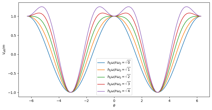
Here we use units so that \(m=r=g=1\), and dimensionless parameters \(\tilde{h}_0\) and \(\tilde{\omega}\). We will consider the limit \(\tilde{\omega} \rightarrow \infty\). From the analysis derived in class, and from the book, we expect the effective potential in this limit to have the form:

\[\begin{gather*} V_{\mathrm{eff}}(\theta) = m\omega_0^2 \cos\theta + \frac{f_1^2}{4m\omega^2} = m\omega_0^2 \cos\theta + \frac{mh_0^2 \omega^2}{4r^2}\sin^2\theta. \end{gather*}\]

th = np.linspace(-2*np.pi, 2*np.pi, 100)
g = r = 1
w0 = np.sqrt(g/r)
fig, ax = plt.subplots(figsize=(10, 5))
for hw2 in [0, 1, 2, 3, 4]:
    V_eff_m = w0**2*np.cos(th) + hw2/r**2*np.sin(th)**2/4
    ax.plot(th, V_eff_m, label=fr'$h_0\omega/r\omega_0 = \sqrt{{{hw2}}}$')
ax.legend()
ax.set(xlabel=r'$\theta$', ylabel=r'$V_{\mathrm{eff}}/m$');

Numerically we will implement these equations in terms of \(\vect{y} = (\theta, \dot{\theta})\), defining a function \(\vect{f}(t, \vect{y})\) such that

\[\begin{gather*} \diff{}{t}\vect{y} = \vect{f}(t, \vect{y}) = \begin{pmatrix} \dot{\theta}\\ \frac{g+\ddot{h}(t)}{r}\sin\theta \end{pmatrix}. \end{gather*}\]

This code generates a figure demonstrating the behaviour of the Kapitza oscillator starting at rest from \(\theta_0=0.1\) for a variety of values \(h_0\omega/r\omega_0\) crossing the threashold at \(\sqrt{2}\). The dashed lines show the simple harmonic motion derived by expanding the effective potential to order \(\theta^2\) and are quite accurate for small initial \(\theta_0\), but start to show deviations for \(\theta_0\gtrapprox 0.2\).

from scipy.integrate import solve_ivp

m = g = r = 1.0
w0 = np.sqrt(g / r)


def h(t, h0, w, d=0):
    """Return the `d`'th derivative of `h(t)`."""
    if d == 0:
        return h0 * np.cos(w * t)
    elif d == 1:
        return -w * h0 * np.sin(w * t)
    else:
        return -w**2 * h(t, h0=h0, w=w, d=d - 2)


def compute_dy_dt(t, y, h0, w):
    theta, dtheta = y
    ddtheta = (g + h(t, h0=h0, w=w, d=2)) / r * np.sin(theta)
    return (dtheta, ddtheta)


h0 = 0.1
y0 = (0.1, 0)
T = 2 * np.pi / w0
t_span = (0, 5 * T)  # 5 oscillations

def fun(t, y):
    return compute_dy_dt(t=t, y=y, **args)

fig, ax = plt.subplots(figsize=(10, 5))

for h0w2 in [0, 1, 2, 3, 4]:
    args = dict(h0=h0, w=np.sqrt(h0w2) / h0)
    res = solve_ivp(fun, t_span=t_span, y0=y0, atol=1e-6, rtol=1e-6)
    ts = res.t
    thetas, dthetas = res.y
    l, = ax.plot(ts / T, thetas, 
                 label=fr'$h_0\omega/r\omega_0 = \sqrt{{{h0w2}}}$')

    # Add harmonic motion predicted by Kapitza formula
    w_h2 = (h0w2/(2*r**2*w0**2) - 1) * w0**2  # See formula below
    if w_h2 >=0:
        ax.plot(ts / T, y0[0]*np.cos(np.sqrt(w_h2) * ts), 
                ls='--', c=l.get_c())
ax.grid(True)
ax.set(xlabel=r'$t/T$', ylabel=r'$\theta$', ylim=(-y0[0], 4 * y0[0]))
ax.legend();

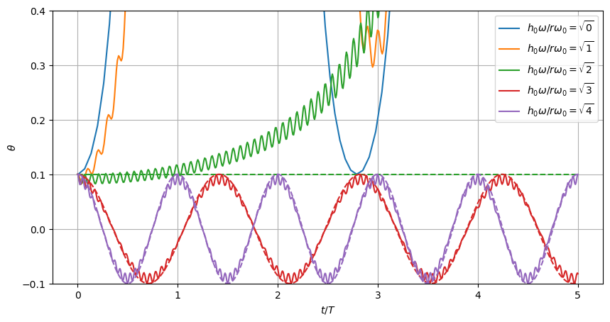
This seems to be consistent with the Kapitza result which says the threshold should be at \(h_0\omega/r\omega_0 = \sqrt{2}\). We have also plotted the predicted harmonic motion (see below) as dashed lines. These start to disagree if we take \(\theta_0 > 0.2\), so we have used a fairly small value of \(\theta_0=0.1\) here but you can play with the code.

Checking Our Work

How might we check our numerical results? The code is pretty simple, but we might have made a mistake with the derivative computation. We can use np.gradient as a quick check.

I found a sign error in the derivative by writing this check. It does not change the results though. To write these checks, it takes a bit of interactive playing to get the correct value of rtol since the finite difference operation has intrinsic errors.

ts = np.linspace(1, 2)
for d in [0, 1, 2]:
    assert np.allclose(
        np.gradient(h(ts, h0=1.2, w=3.4, d=d), ts, edge_order=2), 
        h(ts, h0=1.2, w=3.4, d=d+1), 
        rtol=0.002)

Another possible check is the period of the resultant oscillations. From the Kapitza formula above, we have:

\[\begin{gather*} V_{\mathrm{eff}}(\theta) = m\omega_0^2 \cos\theta + \frac{mh_0^2 \omega^2}{4r^2}\sin^2\theta\\ = m\omega_0^2 \left(1 - \frac{\theta^2}{2}\right) + \frac{mh_0^2 \omega^2}{4r^2}\theta^2 + \order(\theta^4)\\ = \frac{m\omega_0^2}{2}\left(\frac{h_0^2\omega^2}{2r^2\omega_0^2} - 1\right) \theta^2 + \text{const.} + \order(\theta^4)\\ \end{gather*}\]

Thus, we expect an oscillation frequency of:

\[\begin{gather*} \omega_h = \omega_0\sqrt{\frac{h_0^2\omega^2}{2r^2\omega_0^2} - 1} \end{gather*}\]

We include this prediction in our plots above.